BIOFILTERS
In many industrial processes, as well as in emissions collected from bioremediation operations and wastewater treatment plants, the presence of contaminants is observed in the gaseous phase , that is, contained within a gaseous mass. The purpose of biofilters is simply to solubilize these constituents so they can biodegrade through biological mechanisms.
Since the mid-1950s, biofilters have been used to treat gaseous constituents, primarily for odor control, in composting plants and industrial processes. Among the compounds frequently encountered in these applications and effectively treatable, to varying degrees, by biofilters are petroleum hydrocarbons, halogenated and non-halogenated solvents, H₂S, and ammonia. Some specialists disagree, for example, on the feasibility of removing compounds containing nitrogen, e.g., amines, and even ammonia.
As noted earlier, contaminants must be transferred to the liquid phase to allow microbial metabolism. Thus, three stages are distinguished in gas-phase biological treatment:
a. gas-to-liquid phase transfer
b. transport or contact of the constituent with microorganisms
c. biological process proper, conceptually identical
In general, these types of processes have involved fully packed reactors with various types of packing. The first systems, designed for odor control in wastewater treatment plants, frequently used material from the surrounding area and gave rise to the term " soil filters ." These systems operated with extremely low flow rates (CFM per sq. ft. of area or m³/s per m² of area), and with the advent of alternative materials, the term " biofilter" itself emerged. We could conclude this presentation by characterizing this type of reactor by the presence of gaseous constituents and the absence of a moving liquid phase. In the case of biotrickling filters and bioscrubbers , variants of biofilters, to maintain appropriate moisture levels in the filter bed, moisture is supplied through continuous distribution systems , rather than through pre-saturation using a humidification cell.
BRIEF DESCRIPTION OF A BIOFILTER
In general terms, biofilters consist of large tanks through which contaminated air or gas is circulated by forced or induced draft. Shortly after operation, communities or consortia of microorganisms responsible for biodegradation develop on the support medium used (soil, plastics, wood chips).
Some sources indicate that induced draft promotes better air/gas mass distribution. In any case, the pressure drop per meter of packing is generally kept below 10 mmH2O, and pressure drop across the operating system is not a problem except in cases of excessive biomass or liquid accumulation. While the flow rate varies depending on the constituent being treated, 1 to 2 m³/min per m² of area can be considered as preliminary values. Most biofilter installations have focused on odor attenuation or control, but there has been a growing number of applications for VOC removal.
As can be seen in the illustration, the system itself consists of a centrifugal fan or blower, a humidification or saturation system , the biofilter unit itself, and in some cases auxiliary activated carbon systems , either as backup or as a subsequent phase.
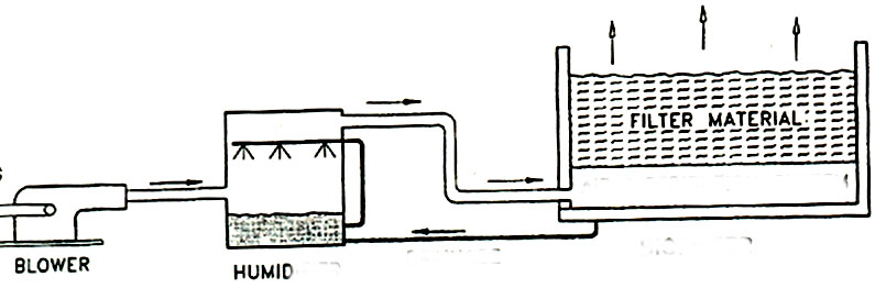
Blower Schematic - Humidification Cell - Biofilter
In many cases, in addition to the humidification system, a manual system is used to add water directly, and some installations utilize condensate return to humidify the biofilter. Generally, the filter media used should offer a large surface area per unit volume, high permeability, and preferably a good intrinsic nutrient source to promote biological processes. Common natural materials include soil, compost, peat, mulch, wood chips, and synthetic materials such as ceramic mounts/random molds, polyethylene Pall rings, and diatomaceous earth pellets. Unlike trickling filters, materials like gravel or stone are not favored due to their low surface area to volume ratio, which results in low processing rates.
APPLICATION # 1: REMOVAL OF 500 PPM TOLUENE BIOFILTER
To properly size a biofilter for treating the gas phase of a vapor volatilization and extraction (VVE) system, several laboratory tests were conducted in a 1 m³ pilot unit. The results of the toluene removal tests in the pilot unit, using compost, are summarized in the following table, which includes the treated flow rate, the initial concentration of the constituent (toluene in this case, with a molecular weight of 92), and the associated removal percentages. By plotting a curve of removal capacity (g/h * 3) versus applied VOC load (g/h * 3), the preliminary sizing for a full-scale installation with a flow rate of Q = 3 m³/min and a toluene concentration of 500 ppm is to be performed.
| Q m3/min | Q m3/h | Q m3/s | CFM | inlet ppm | MW | e % |
| 1 | 60 | 0.017 | 35,315 | 16 | 92 | 99 |
| 0.5 | 30 | 0.008 | 17,657 | 164 | 92 | 99 |
| 0.67 | 40.2 | 0.011 | 23,661 | 151 | 92 | 99 |
| 0.33 | 19.8 | 0.006 | 11,654 | 366 | 92 | 98 |
| 1.1 | 66 | 0.018 | 38,846 | 122 | 92 | 96 |
| 0.67 | 40.2 | 0.011 | 23,661 | 228 | 92 | 94 |
| 0.8 | 48 | 0.013 | 28,252 | 213 | 92 | 92 |
| 0.7 | 42 | 0.012 | 24,720 | 277 | 92 | 90 |
| 0.75 | 45 | 0.013 | 26,486 | 290 | 92 | 88 |
| 0.67 | 40.2 | 0.011 | 23,661 | 357 | 92 | 83 |
| 0.75 | 45 | 0.013 | 26,486 | 384 | 92 | 75 |
| 0.45 | 27 | 0.008 | 15,892 | 681 | 92 | 67 |
| 0.85 | 51 | 0.014 | 30.017 | 389 | 92 | 60 |
| 1 | 60 | 0.017 | 35,315 | 366 | 92 | 57 |
| 0.67 | 40.2 | 0.011 | 23,661 | 551 | 92 | 55 |
| 0.7 | 42 | 0.012 | 24,720 | 518 | 92 | 52 |
| 0.8 | 48 | 0.013 | 28,252 | 523 | 92 | 50 |
| 1.1 | 66 | 0.018 | 38,846 | 380 | 92 | 48 |
| 0.9 | 54 | 0.015 | 31,783 | 451 | 92 | 46 |
| 0.8 | 48 | 0.013 | 28,252 | 579 | 92 | 44 |
| 0.85 | 51 | 0.014 | 30.017 | 585 | 92 | 43 |
| 0.67 | 40.2 | 0.011 | 23,661 | 762 | 92 | 41 |
| 0.85 | 51 | 0.014 | 30.017 | 643 | 92 | 39 |
| 0.67 | 40.2 | 0.011 | 23,661 | 819 | 92 | 36 |
| 0.67 | 40.2 | 0.011 | 23,661 | 909 | 92 | 34 |
We will illustrate the calculations involved in a "manual"/step-by-step manner only for the first set of data. The results for all cases, necessary for the graph, are detailed in the complete spreadsheet included below.
For convenience, let's anticipate conversions and express the air flow rate Q in different units:
Q = 1 m3/min = 35.3145 CFM = 60 m3/h = 0.017 m3/s
Given an initial toluene concentration of Ci = 16 ppm, and a molecular weight of 92, we can calculate the corresponding flow, namely
g mole / min = 35.3145 CFM * 16 ppm * 28.3 / (10^6*22.4) = 0.00071 g mole / min = 7.1386 e-04 g mole / min =
7.1386 e-04 g mole / min * molecular weight = 7.1386 e-04 g mole / min * 92 = 0.065675 g/min
Given that the volume of the biofilter is 1 m3, we can easily calculate the applied load LR , i.e.
applied load LR = VOC loading rate = Q * Ci / V = 0.065675 g/min * 60 min/h / 1 m3 = 3.94 g / h per m3
Given that they indicate a removal efficiency of E = 99%, the removal capacity EC is given by:
removal capacity EC = Q * (Cf - Ci) / V = Q * ( Ci * E / 100) * V = ( Q * Ci / V) * E / 100 = LR * E /100 = 3.9 * 99 / 100 = 3.9 g / h per m3
Similarly, we obtain all the other Lr and EC pairs necessary to create the graph and estimate the maximum elimination capacity ECmax. The table below shows all the required calculations.
| VOC loading | VOC loading | verification | |||||||||||||||
| rate | rate | EC | EC | Lm | EC | ||||||||||||
| Q m3/min | Q m3/h | Q m3/s | CFM | inlet ppm | MW | e % | g mole /min | g/min | mg/min per m3 | g/h per m3 | g/min * m3 | g/h per m3 | g/h per m3 | g/h per m3 | |||
| 1 | 60 | 0.017 | 35,315 | 16 | 92 | 99 | 0.00071386 | 0.065675 | 65.67488 | 3.9 | 0.065 | 3.9 | 3.5 | 3.9 | |||
| 0.5 | 30 | 0.008 | 17,657 | 164 | 92 | 99 | 0.00365852 | 0.336584 | 336.5838 | 20.2 | 0.333 | 20.0 | 17.9 | 20.0 | |||
| 0.67 | 40.2 | 0.011 | 23,661 | 151 | 92 | 99 | 0.00451381 | 0.41527 | 415.2705 | 24.9 | 0.411 | 24.7 | 22.1 | 24.7 | |||
| 0.33 | 19.8 | 0.006 | 11,654 | 366 | 92 | 98 | 0.00538873 | 0.495763 | 495.7633 | 29.7 | 0.486 | 29.2 | 26.4 | 29.2 | |||
| 1.1 | 66 | 0.018 | 38,846 | 122 | 92 | 96 | 0.00598748 | 0.550848 | 550.8481 | 33.1 | 0.529 | 31.7 | 29.3 | 31.7 | |||
| 0.67 | 40.2 | 0.011 | 23,661 | 228 | 92 | 94 | 0.00681555 | 0.627031 | 627.0309 | 37.6 | 0.589 | 35.4 | 33.3 | 35.4 | |||
| 0.8 | 48 | 0.013 | 28,252 | 213 | 92 | 92 | 0.00760258 | 0.699437 | 699.4375 | 42.0 | 0.643 | 38.6 | 37.2 | 38.6 | |||
| 0.7 | 42 | 0.012 | 24,720 | 277 | 92 | 90 | 0.00865106 | 0.795897 | 795.8975 | 47.8 | 0.716 | 43.0 | 42.3 | 43.0 | |||
| 0.75 | 45 | 0.013 | 26,486 | 290 | 92 | 88 | 0.009704 | 0.892768 | 892.7679 | 53.6 | 0.786 | 47.1 | 47.5 | 47.1 | |||
| 0.67 | 40.2 | 0.011 | 23,661 | 357 | 92 | 83 | 0.01067172 | 0.981798 | 981.7984 | 58.9 | 0.815 | 48.9 | 52.2 | 48.9 | |||
| 0.75 | 45 | 0.013 | 26,486 | 384 | 92 | 75 | 0.01284943 | 1.182148 | 1182.148 | 70.9 | 0.887 | 53.2 | 62.8 | 53.2 | |||
| 0.45 | 27 | 0.008 | 15,892 | 681 | 92 | 67 | 0.0136726 | 1.257879 | 1257.879 | 75.5 | 0.843 | 50.6 | 66.9 | 50.6 | |||
| 0.85 | 51 | 0.014 | 30.017 | 389 | 92 | 60 | 0.01475231 | 1.357212 | 1357.212 | 81.4 | 0.814 | 48.9 | 72.1 | 48.9 | |||
| 1 | 60 | 0.017 | 35,315 | 366 | 92 | 57 | 0.01632949 | 1.502313 | 1502.313 | 90.1 | 0.856 | 51.4 | 79.9 | 51.4 | |||
| 0.67 | 40.2 | 0.011 | 23,661 | 551 | 92 | 55 | 0.01647092 | 1.515325 | 1515.325 | 90.9 | 0.833 | 50.0 | 80.5 | 50.0 | |||
| 0.7 | 42 | 0.012 | 24,720 | 518 | 92 | 52 | 0.01617779 | 1.488357 | 1488.357 | 89.3 | 0.774 | 46.4 | 79.1 | 46.4 | |||
| 0.8 | 48 | 0.013 | 28,252 | 523 | 92 | 50 | 0.01866737 | 1.717398 | 1717.398 | 103.0 | 0.859 | 51.5 | 91.3 | 51.5 | |||
| 1.1 | 66 | 0.018 | 38,846 | 380 | 92 | 48 | 0.01864952 | 1.715756 | 1715.756 | 102.9 | 0.824 | 49.4 | 91.2 | 49.4 | |||
| 0.9 | 54 | 0.015 | 31,783 | 451 | 92 | 46 | 0.01810967 | 1.66609 | 1666.09 | 100.0 | 0.766 | 46.0 | 88.6 | 46.0 | |||
| 0.8 | 48 | 0.013 | 28,252 | 579 | 92 | 44 | 0.02066617 | 1.901288 | 1901.288 | 114.1 | 0.837 | 50.2 | 101.1 | 50.2 | |||
| 0.85 | 51 | 0.014 | 30.017 | 585 | 92 | 43 | 0.02218535 | 2.041052 | 2041.052 | 122.5 | 0.878 | 52.7 | 108.5 | 52.7 | |||
| 0.67 | 40.2 | 0.011 | 23,661 | 762 | 92 | 41 | 0.0227783 | 2.095603 | 2095.603 | 125.7 | 0.859 | 51.6 | 111.4 | 51.6 | |||
| 0.85 | 51 | 0.014 | 30.017 | 643 | 92 | 39 | 0.02438492 | 2.243413 | 2243.413 | 134.6 | 0.875 | 52.5 | 119.2 | 52.5 | |||
| 0.67 | 40.2 | 0.011 | 23,661 | 819 | 92 | 36 | 0.02448219 | 2.252361 | 2252.361 | 135.1 | 0.811 | 48.7 | 119.7 | 48.7 | |||
| 0.67 | 40.2 | 0.011 | 23,661 | 909 | 92 | 34 | 0.02717254 | 2.499873 | 2499.873 | 150.0 | 0.850 | 51.0 | 132.9 | 51.0 | |||
Next, we simply transcribe the abscissas and ordinates in order to easily obtain the graph.
|
|||||||||||||||||
|
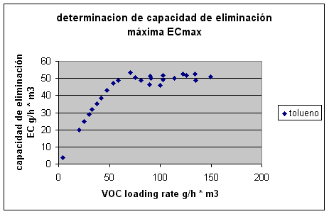
A fairly characteristic behavior can be observed for this constituent within the considered applied load range. From direct observation/assessment of the curve, we can estimate an ECmax on the order of 50 g/h per m³ . Simply recalculate for the real-scale case requested, ie 3 m3/min and 500 ppm Q = 3 m3/min = approx. 106 CFM Given an initial toluene concentration of Ci = 500 ppm, and a molecular weight of 92, we can calculate the corresponding flow, namely g mole / min = 106 CFM * 500 ppm * 28.3 / (10^6*22.4) = 0.067 g mole / min = 0.067 g mole / min * molecular weight = 0.067 g mole / min * 92 = 6.157 g/min The required volume will then be V = 6.157 g/min * 60 min/h / ECmax = 6.157 g/min * 60 min/h / 50 50 g / h per m3 = 7.4 m3 In practice, a volume would be designed, for example, between 30 and 70% larger. |
APPLICATION # 2: HYDROCARBON REMOVAL BIOFILTER (TPH = 130 ppm )
A soil bioremediation plant using volatilization and vapor extraction generates approximately 1500 CFM with a total hydrocarbon (TPH) content of around 130 ppm. The goal is to estimate the water inputs required at different stages, i.e., the humidifier tank and the biofilter itself, to ensure optimal conditions for biological activity and subsequent component assimilation. The gas phase temperature is estimated at approximately 47°C (116.6°F) with a relative humidity of 20%. For the purposes of performing the balances, the system will be approximated as steady state, assuming the unit discharges at 100% saturation.
While we won't deny that there will be some number crunching, primarily to express the magnitudes in units convenient for everyone, the solution to the problem essentially boils down to just three (3) simple readings from a psychrometric chart , a classic in air conditioning. Although we will present the psychrometric information in detail, we offer below an illustrative version that will serve to visually corroborate the numerical calculations we will be developing.
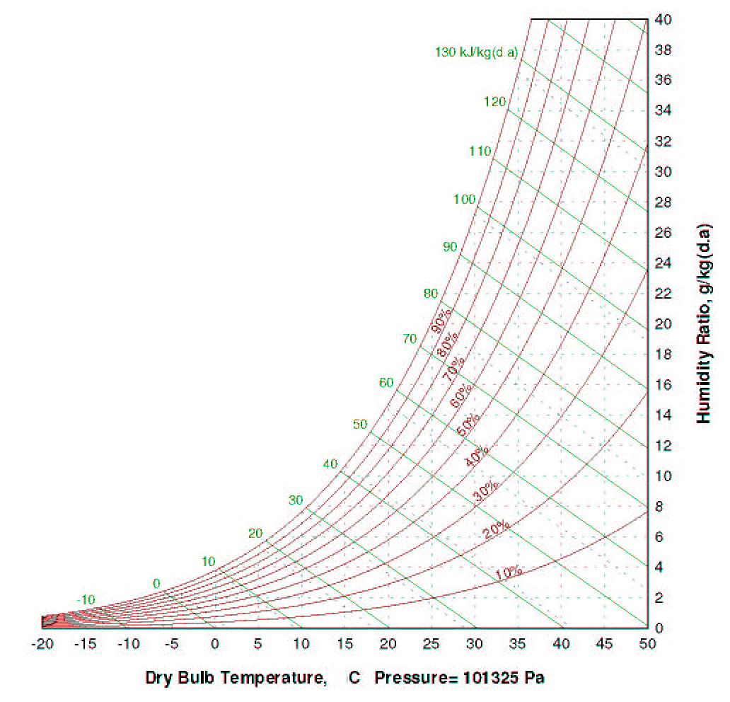
Psychrometric chart in SI units
The water addition or replenishment at each stage (humidification cell, biofilter) will be determined primarily by comparing the moisture content at the inlet and outlet, respectively. To solve this problem, we will not rely on the chart but rather on the repeated application of the ASHRAE HVAC 2 Toolkit . Although it consists of a set of algorithms and subroutines written in Fortran , the practicality of the small modules will facilitate the gradual presentation of results, both intermediate and final.
The specifications indicate a dry-bulb temperature of 47°C and a humidity level of 20% for the gas phase . Therefore, upon entering the humidification cell , the air or gas has the following properties:
| 47 | °C | 116.6 | °F | W = | 0.013323 | 93.3 | grH2O/lbDryAir | 0.013323 | lbH2O/lbDryA | |
| 0.2 | RH | 20 | % | H = | 81733.4 | 43.7 | btu/lb Dry Air | |||
| 101325 | Patm | RhoD = | 1.07943 | 0.0674 | lb/cu.ft. | |||||
| Twb = | 26.4823 | °C |
If the humidification cell "functions correctly," the air passing through the cell will absorb moisture, exiting 100% saturated and following a straight line towards the point on the saturation curve corresponding to the indicated wet-bulb temperature, approximately 26.5°C (26.4823°C). This is in accordance with the water temperature in the humidification cell circuit, which may need to be increased to balance the biofilter's outlet requirements and maintain saturation at all points in the circuit. Otherwise, the biofilter will dry out or collapse as it absorbs moisture from the support, packing, or bed intended for the biomass.
The second reading corresponds to the psychrometric chart, or in our case, using the calculation routines to determine the air conditions at the outlet of the humidification cell , which we will assume to be identical to the inlet of the biofilter . Imposing a dry-bulb temperature of approximately 26.5°C (26.4823°C), 100% saturation results in:
| 26.4823 | °C | 79.7 | °F | W = | 0.021992 | 153.9 | grH2O/lbDryAir | 0.021992 | lbH2O/lbDryA | |
| 1 | RH | 100 | % | H = | 82694.2 | 44.2 | btu/lb Dry Air | |||
| 101325 | Patm | RhoD = | 1.13782 | 0.0710 | lb/cu.ft. |
The input required by the humidification cell to achieve saturation of the discharge is calculated directly by the difference in moisture content between the two points considered, that is:
Dry air mass = 1500 CFM * 0.0674 lb/cu.ft. = 101.1 lb/min dry air
Required input Humidification Cell Stage = (153.9 grH2O/lbDryAir - 93.3 grH2O/lbDryAir) * 101.1 lb/min dry air = 6126 gr/min = 6126 gr/min * 60 min/h / 7000 gr/lb = 52.5 lbH2O/hr = 52.5 lbH2O/hr / 8.33 lb/gal = 6.31 gal/h = approx. 23 L/h (humidification cell)
With some simplifications, we are now ready to examine the biological oxidation process of the 130 ppm of TPH contained in the gas phase to be treated. For the purposes of stoichiometric calculations, we will assume it is appropriate to approximate the 130 ppm of TPH as 130 ppm of hexane (C6H14). We will then calculate the heat input and water generation resulting from the biological oxidation of this component.
Using a table (e.g., Himmelblau.652) or "calculation", we can easily obtain the molecular weight of hexane, i.e.:
PM hexane = PM C6H14 = 6 * 12 + 14 * 1 = 86
There is practically no difference between the molecular weight of dry air (29) and air under the given conditions (28.8), so based on the mass flow rate of dry air we can easily calculate the flow rate or mass of hexane entering the system, that is:
Mhex = ( 130 ppm / 10^6) * PMhex / PMair * 101.1 lb/minDryAir = ( 130 / 10^6) * (86/29) * 101.1 lb/minDryAir = 0.039 lbHex/min
Since we can approximate the heat generated in the biological oxidation of hexane as the heat of combustion of said constituent (ca. 19385 btu/lb) we can immediately calculate the enthalpy of the biofilter discharge from the sum of the enthalpy at the inlet conditions plus said increase, that is:
Heat input from hexane biodegradation per pound of dry air = 0.039 lbHex/min * 19385 btu/lbHex / 101.1 lb/min dry air = approx. 7.5 btu/lbDryAir
Biofilter gas phase discharge enthalpy = inlet enthalpy + biological input = 43.7 btu/lbDryAir + 7.5 btu/lbDryAir = approx. 51.2 btu/lbDryAir
The third and final consultation of the psychrometric chart, specifically the enthalpy reading on the saturation curve, indicates that this enthalpy value corresponds approximately to a temperature of 30°C , give or take a decimal. The resulting numerical calculation from the routines in the Ashrae/HVAC Toolkit confirms the results obtained, with the following conditions for the planned discharge of the biofilter :
| 30 | °C | 86.0 | °F | W = | 0.027204 | 190.4 | grH2O/lbDryAir | 0.027204 | lbH2O/lbDryA | |
| 1 | RH | 100 | % | H = | 99690 | 51.5 | btu/lb Dry Air | |||
| 101325 | Patm | RhoD = | lb/cu.ft. |
Similarly, we can estimate the water input required to maintain a saturated outlet of the biofilter without affecting or subtracting moisture content from the biofilter bed or filling.
Required contribution Biofilter Stage = (190.4 grH2O/lbDryAir - 153.9 grH2O/lbDryAir) * 101.1 lb/min dry air = 3690 gr/min = 3690 gr/min * 60 min/h / 7000 gr/lb = 31.6 lbH2O/hr = 31.6 lbH2O/hr / 8.33 lb/gal = 3.80 gal/h = ca. 14.4 L/h (biofilter)
It is advisable to replicate the calculations for different data sets, for example, by increasing the inlet air temperature or the water circuit temperature of the humidification cell, and to examine the impact on the energy inputs required at each stage. In practice, it may or may not be feasible/appropriate to implement modifications that increase the energy inputs to the system as required.
Finally, the careful reader may speculate on the water values generated by the biological oxidation process within the biofilter of the various hydrocarbons, approximated as a single constituent, hexane in this case. However, the oxidation of 130 ppm of hexane, taking into account its corresponding mass flow rate (Mhex), produces barely
Mhex * 6 * PMH2O / PMhexane = 0.039 lbHex/min * 6 * 18 / 86 = 0.049 lbH2O/min
This, when referred to the mass of dry air (101.1 lb/min dry air), results in = 0.049 lbH2O/min / 101.1 lbDryAir/min = 0.00048 lbH2O/lbDryAir versus the corresponding calculated requirement for the biofilter, i.e. = 31.6 lbH2O/hr / (60 m/h * 101. lbDryAir/min) = 0.0052 lbH2O/lbDryAir
To visualize the evolution through the system, we have included the worksheet that summarizes the calculations performed.
In order to obtain more information and/or request courtesy capacity plannings or case assessments, please send us an e-mail to answers@engineeringfundamentals.com cc.: balestie@umich.edu.
It is recommended to include a brief initial description of the case, ideally no more than one page, or project in progress / under study. The possibility of receiving and handling individual technical consultations has been foreseen but are limited as per availability. Alternatively make contact later on via sms/telephone +1 917 300 3024